Category: COVID-19

The chart above is the one I’ve been thinking about putting together for quite a while now. It’s really busy, but it has a ton of information in it. Here’s how to read it.

1. Normalizing Case Counts by Population: I’m comparing both Pima and Maricopa counties (the two largest in the state by far) on a cases per 1000 basis. Why do I do this? If I compare them on raw numbers of cases, it looks like Pima County is doing SO much better than Maricopa because they have 1/4 the cases. However, Pima also has 1/4 the population. This is one way the news media exaggerates stories, probably because it looks stark and dramatic when you don’t compare appropriately. When I do this the right way, you can see that Pima and Maricopa had the same exact slope (more or less) up until Memorial Day. This is the purple arrow. After memorial day, we see case growth accelerate in both counties but a good deal faster in Maricopa County. This is the source of much of the overall case growth in Arizona.
2. Polynomial Trend Lines: The fat, light blue and pink lines are the trend lines for Maricopa and Pima respectfully. These are both modeled with 3rd Order Polynomials, which essentially means that the formula to create the trend line is something like Ax^3 + Bx^2 + Cx + D. This essentially shows that the case growth is accelerating (curving upward). Almost every state’s case growth right now can be modeled with this same kind of function. The trend line allows us to do simple predictions for the next few days on what the case growth might be. It is not a good predictor for much more than a few days out because the situation is too complex for that.
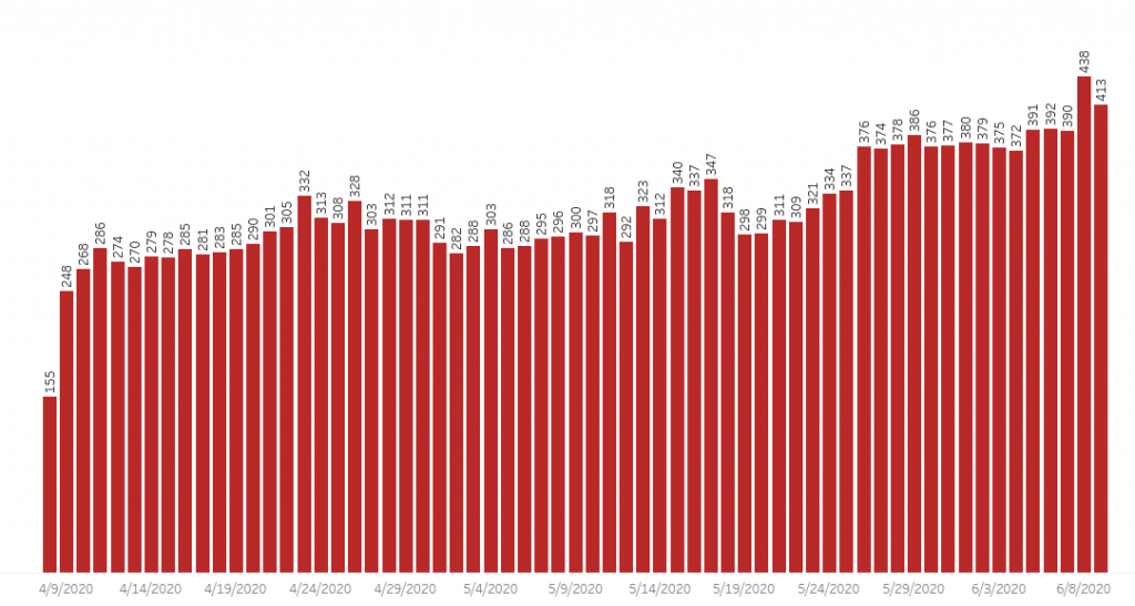
3. Testing Numbers and Results: The yellow dashed line represents the numbers of tests on each day. I had to pull these numbers from the state’s online Dashboard manually because they won’t let us download it. So the data may be off by 5-10 tests per day. Note that the Test Numbers are represented on the secondary Y-axis (the one on the right). This can be confusing, but it allows me to provide more valuable visualizations. I also tried to capture the weekly percent positive for the tests. As you can see the percent of tests that are positive is growing. I’ll try to offer some possible explanations for that in my conclusion.
4. Data Lags: Note that I extend the blue “Stay at Home” rectangle about 10 days past the 5/17 expiration date. I do this to demonstrate that most of the data we see every day has the potential for being as much as 10 days old. Data collection isn’t very clean and efficient when dealing with health-related issues. Any time you look at COVID-19 data, whether it is the CDC or the WHO or the AZ DHS, you need to remember that it’s likely reporting the state from a week or so beforehand. I’ve seen some embarrassing data analyses during this outbreak by professional media that did not account for the fact that recent data is likely to be underreported due to this lag. The testing numbers above are a good result. I have no reason to believe that AZ has slowed testing in the last week. We just don’t have the accurate numbers in yet.
5. Events/Triggers: I’ve labeled various events and triggers on the chart. The stay at home order and its expiration are interesting, as is Memorial Day. Face Masks became mandatory in AZ on about 6/20. You can be sure that will be added as an important event as the time goes on and more data comes in. My expectation is that we’ll see some sort of change in the trends in late June or early July (to account for the data lag but also the 14 day hospitalization cycle time).
6. Hospitalization: I’m not including hospitalization stats in this chart, largely because first, the chart is already too busy, but second, I have a hard time trusting/believing the states and counties hospitalization data, which all seem to contradict one another. Suffice it to be said that right now hospitals in the state are jam packed with COVID cases and there’s not much margin (at least in the traditional sense).

Analysis of the Chart

1. Comparison of Pima and Maricopa Cases per 1000: As mentioned above, it’s very interesting to me that the case growth up until Memorial Day in both counties is essentially linear and basically the same slope. Ending the stay at home order doesn’t seem to have dramatically impacted this case growth rate (even considering the data lag). Two events seem to have occurred simultaneously that may be causal for the dramatic case growth lately. First is Memorial Day. We see the exponential case growth start a few days after Memorial Day. It may well be that a number of people contracted the virus during Memorial Day activities (we’ll probably never know if the protests/riots contributed due to bad data on those events). Maybe there were super-spreader events during the holiday too that we haven’t identified. The second major event that certainly contributes is the doubling of testing that also started about this same time. The state was conducting an average of about 8K tests per day up until about June 4th when it doubled this to an average of about 16K tests per day. During the stay at home period there was an extreme bias in the tests toward sick patients because one could barely get tested unless they exhibited symptoms. Even then, only about 5% of tests were positive. The spreading that may have occurred around Memorial day combined with the doubling of testing have resulted in not just doubling the number of cases, but exponential growth, because now the percent positive rates are approaching 20%.
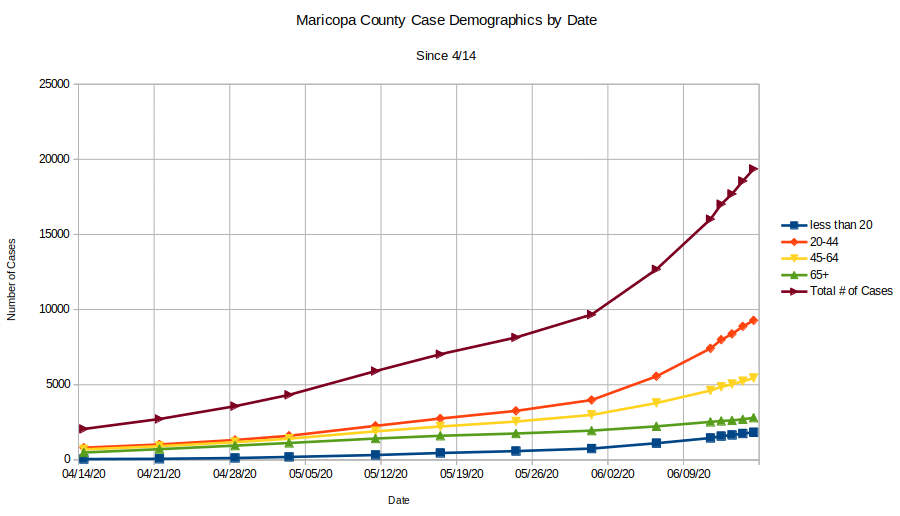
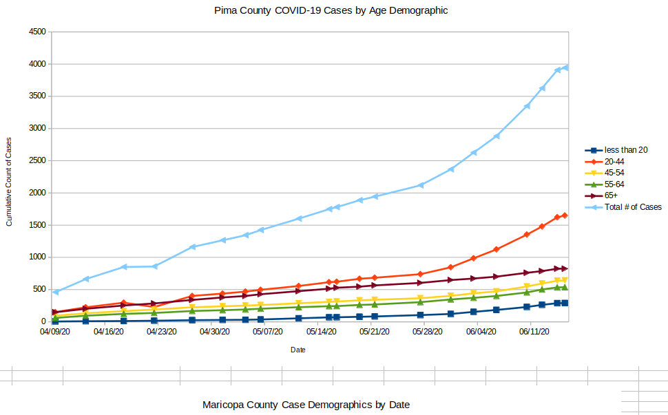
2. Why are the Tests’ positivity rates so high? This is interesting to think about but here are a few possible reasons. First: There is a lot more virus out there now since Memorial Day and people are catching it. One telling stat is what I have shown a few times (which still holds) that shows that the growth rate of infections in the 65+ community is still the same now as it was during the stay at home order. In short, this demographic is still travelling down the same purple arrow! All other groups are reflecting the exponential growth trend. It is likely that the 65+ community is being just as careful now as they did during stay at home orders (and maybe group homes have also become more careful) and they’re avoiding the bloom in the virus. Everyone else is exposed to a larger population of the virus. This is speculation, but it makes sens. Second: It may well be that there is emerging another kind of testing bias and now people who are more likely to be infected are more likely to get tested. For instance, since I can’t see WHERE the tests are being conducted, there’s a chance that a higher percentage of tests are coming from regions that are already having major outbreaks (border counties, native communities). This is possible, especially given that there appears to be clear indications that the virus is more prevalent in some areas than others. The only way to really prevent this bias is to do what some European countries did and randomize testing. Otherwise we have no real idea of what’s happening. Third point: I’m convinced that we’re not seeing issues with false positives on the PCR tests (but I still believe there are high false positives on the antibody tests that make them somewhat less informational right now).
3. Why are the Rates different for Pima and Maricopa County? First, one thing we’re seeing is that the rates can be very different in different regions. Not just across the world or across US states, but even by AZ Zip codes. After about 3 weeks of tracking this I’m still seeing the less wealthy zip codes have the highest overall numbers of cases per 1000 people AND the highest growth rates over time. This is interesting to analyze because it makes one curious about why this is happening. There are a number of hypotheses for this. It’s possible that people who are overall less healthy (maybe they don’t have good health care) may be more likely to get infected and then need to seek medical care. However, it does appear that this isn’t a very solid hypothesis when one looks at the demographics where the largest number of cases by far is in the younger, healthier age groups. Culture is one hypotheses I hear, for this, where the cultures in less wealthy regions have evolved to rely on others much more than the cultures in wealthy regions require. There are also ethnic cultures and traditions that may have some causality. Also, based on this evidence, some of the activities that are more commonly engaged in the wealthier zip codes (dining out, going to the gym, etc.) may actually be less causal of infections than we thought. From my observation, also, the culture of mask wearing in Arizona is stronger in the wealthier zip codes than in less wealthy or rural zip codes. It’s possible that this has an impact, but time will tell how significant of one. Regardless, there’s still much to learn about this.
4. Case Severity: With this virus, just like with the flu, there is a very wide range of severity. Measuring cases is interesting from a numbers standpoint, but it is not a good representation for the severity of an outbreak. A very large majority of the new cases we’ve been measuring (and in some cases, stressing about) are asymptomatic (or low-symptomatic) cases that aren’t requiring medical attention. The better measure of severity is deaths, of course, but also hospital cycle times and capacity measures (because they’re leading indicators for deaths). The hospital measures are extremely hard for a number of reasons mentioned in an earlier article on this site… Hospitals and their staffs are clearly being stressed with the growth in severe cases (even thought this growth is very small compared to the asymptomatic cases). Some of this is because this disease forces a 2-plus week cycle time on cases, something that appears to be extremely unusual for viral infections.

The Effect of Wealth on Cases in a Region

Above is the latest comparison of COVID-19 cases per 1000 population compared to median income. Note that the lowest median income zip codes is on the left and the highest is on the right. The average number of cases per 1000 for the poorest 25 zip codes is 9. The average for the wealthiest 25 zip codes is 2.6. You can see the yellow trend line shows a decrease in cases from the left to the right (case counts are on a logarithmic scale on the right y-axis). The red line are actual cases per 1K for the zip codes. Note that you may not see your zip code labeled on the chart (only about every 10th zip are labeled because otherwise the chart would extend around the room!).

Case growth follows this exact same trend. This means that the regions with the highest rate of change in their case counts (hot spots) tend to be on the left of this chart. This indicates that the overall trend of more cases in less weathy areas is not changing.

The Effect of Population Density

One explanation for the “wealth effect” is population density. This makes sense in light of the now-ubiquitous 6 Feet of Separation. Many of the lower income areas with high outbreaks are in zip codes that are known to have large numbers of people living in dense environments (apartment complexes, for instance). However, some of the regions with the highest outbreaks are rural and agricultural regions that have very low population density.

Overall, however, the chart above does show that the cases per 1K tends to go up as population density increases. The trend line is fit with an exponential function that has a decent (but not ideal) fit. Most likely, density is one component of the problem, but is likely not one of the larger components.

The Effect of Median Age

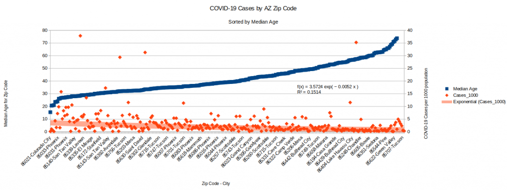
Another interesting characteristic of some zip codes that may be driving higher case counts is median age. This makes sense, especially since we already know that most of the cases in the current outbreak are asymptomatic cases among younger people. Therefore, this chart tells a very clear story. Outbreaks are much higher in regions with lower median ages.

I’ve been fascinated throughout this outbreak at how it breaks across latitude ranges. Here’s the latest info on Latitude.

The above chart shows cumulative numbers normalized by the population for each region. This shows the upper North latitudes continue to lead in total cumulative cases and deaths per 1000 persons but a couple of the South latitude ranges are starting to catch up (Brazil, Ecuador, Chile, Argentina, South Africa).

Notably, the middle latitude ranges are still far less affected cumulatively.

Now above we see the instantaneous rates of change across the latitude bands. This chart shows us where today’s hot spots are. Note that the US latitudes are very low because overall, US cases are low compared to population. Most of the US cases right now are happening in the 30-40 N Latitude range (Arizona, Texas, California), but the rates in these locations are not large enough to show a significant spike in instantaneous rates (which are spiking for Africa and South America across the board right now). Note that 20-30 N. Latitude are starting to show increased slope in cases and deaths. This is largely due to a growing number of cases in India and Bangladesh.

Hospitalization data right now seems to be one of the most critical signals that a COVID-19 outbreak in a region is getting serious. However, hospitalization data is really hard to analyze for a number of reasons:

1. Hospitals don’t like to share data. In many cases in the United States (including Arizona) there was no hospitalization data during the first part of COVID-19. This was not the case with European countries. I can make a number of guesses about this including Health Information Privacy (HIPAA), inconsistent data collection, and even a sense of unwillingness by private and public hospitals alike to reveal too much about their business. However, with COVID-19 there seems to be a renewed sense that hospitals are a public good and need to be more transparent. Arizona has a new executive order (23-2020) governing the reporting of COVID-19 data.
2. There doesn’t seem to be a strong central governance around hospitalization data. Before COVID-19 this was always what I assumed that CDC did, but now I think it’s just a function of the state’s Health Department. I think that if CDC created guidelines and reporting rules, we would have much richer and much more predictive data sets around the health of people in the US. Until then, however, it requires someone to clean data, hand-build datasets, etc., to extract useful information.
3. Hospital data tends towards the anecdotal side. I have had many forwards from people on LinkedIn or Facebook that came from the cousin of their sister-in-law, who is a surgeon in New York explaining how overwhelmed the ICU is there in whatever town they serve. Then an hour later I get another forward from some connection in the very next county in New York explaining why their hospital has no COVID cases. This is very, very common. I think some of this is due to the above lack of transparency in hospitals, where data is even hidden from employees. I’ve had more than one person who works in a hospital in Arizona tell me at some point during the COVID-19 outbreak that there is only around XX people in the COVID ward right now — “But don’t tell anyone”. I don’t understand the perceived secrecy of this data, but due to the secrecy and poor data reporting, the ancecdote tends to carry the day. Until the next day when the opposite story comes out.
4. Hospitalizations classified as COVID-19 may not have initially sought treatment for COVID. Florida is starting to run into a new kind of COVID-asymptomatic hospital patient who seeks care for an unrelated issue (broken leg, etc.) and then is tested and found to have COVID-19. This is challenging. Does the patient need to go to the COVID ward? Initially, it seems that yes, they were, but now the state is starting to handle these patients differently (and save the COVID ward for those with COVID symptoms). This is unlikely to be affecting ICU bed numbers, of course, but is possibly affecting inpatient bed counts (which are already reaching maximums as well).
5. The hospital business and processes are not well understood by the layman, even by the hospital employee at times. This results in lack of understanding of the real meaning behind a data visualization.

Overview of Arizona ICU Bed Management during COVID-19

One thing that is very interesting to me is ICU bed management. Obviously hospitals want to leverage their invested ICU bed capital to make money. This would seem to require limited excess capacity in the ICU — i.e., most beds full most of the time. During COVID-19 one of the earlier stories was how COVID would overrun the ICU’s at most hospitals. I believe this did happen to an extent in New York, but it hasn’t happened yet in Arizona. COVID-19 patients are still less than 40% of all the ICU beds occupied in Arizona, but the number has been growing. See the chart below which compares the percentage of all occupied ICU beds that have a COVID-19 patient in them.

Thoughts:

1. It seems like the COVID patients peaked as a percentage of the total ICU bed population in mid-April and then gradually tapered off until the lockdown easing was fairly much complete. We then see acceleration in cases drive up the percentage of COVID-19 patients to near 40%. Note there is still 15+% unoccupied ICU beds (though I’m not sure if they’re in the right places). But clearly, whoever the non-COVID patients in the ICU are, they’re decreasing. There may be an element of elective surgeries in the non-COVID ICU population, but I don’t think they’re as many as usual.
2. I can’t fully get my arms around what this chart is telling me, other than perhaps it shows that hospitals know how to manage their ICU bed resources. The total percentage of ICU beds filled in the state has gone from 74% around 5/21 to about 85% today (total about 130 beds). They have done this while COVID-19 cases in the ICU have increased by about 230 people (hence, the now-higher percentage of COVID patients in ICU beds). I don’t know how they made up those extra 100 people, but they did it somehow. They have some margin to work with, I suppose, because even today, 60+% of all inhabitants of the ICU are non-COVID.
3. This management is why the increase in hospital bed numbers has been linear while the COVID-19 case growth has been exponential. Here’s a view of hospitalization just compared with the numbers of 65+ COVID-19 cases. Note that the 65+ group which looks pretty linear when compared to the 20-44 age group cases still looks exponential when compared to the hospitalization (especially the ICU) rates.

The state AZHS Dashboard provides a download and a map of COVID-19 Cases by Zip code. I was playing with the data and noticed that most of the regions with higher cases per 1000 were areas that were known to have lower median incomes. This intrigued me, because we really don’t know much about who is involved in this current wave of COVID-19 infections (other than the age demographics that I presented in previous articles).

COVID-19 Outbreak Info by the richest and poorest zip codes in Arizona

First caveat… due to tribal regulations, I have zero data for tribal regions, many of which would qualify as areas with very low median incomes. This is too bad and if anyone from these regions is interested in having their data analyzed securely, please contact me.

My thoughts on this chart:

1. It is pretty clear that COVID-19 outbreaks are much higher in Zip Codes with lower median incomes. The yellow trend line on the chart shows a R2 score of just under 0.5, which indicates that the trend is a pretty solid fit considering this is real-world data. The average number of cases per 1000 in the poorest 20 zip codes is over 9 and the average of cases per 1000 for the richest 20 zip codes is 1.9. Even if you subtract the Yuma and Nogales zip codes that have some of the highest case rates in the country, the average for the 20 poorest zip codes is 6.5. I posted this chart on Facebook looking for theories on why the situation is this pronounced. There was a lot of good discussion about this, and it is clear that whatever is causal for this disparity, it is comprised of multiple cultural and economic variables.
2. Lots of businesses that were shut down during the state’s COVID-19 lockdown (gyms, restaurants, and even churches) probably have a much higher representation in the wealthier zip codes, where very large gyms, restaurants, and churches thrive. This would be an interesting study. It does seem like the current outbreak probably has much less to do with these kinds of businesses than we would have guessed.
3. Some of these regions that have much higher cases per 1000 people are agricultural areas. Most of these particular regions also have a very low death rate. Perhaps there’s something they’re doing that makes them more likely to get infected but less likely to be badly affected.
4. I also suspect that one influential variable is mask usage. My observation in Tucson is that the Foothills region has been much more diligent around face coverings than other parts of Tucson (and certainly rural Arizona). This may be one reason the Tucson Foothills zip code COVID-19 cases per 1000 are extremely low. This may also apply to regions in Phoenix that are similar to the Tucson Foothills.
5. Now that Pima and Maricopa county are mandating face coverings in public, we have a great opportunity for a natural experiment on the value of Face Coverings. My guess would be that we’ll see the case count flatten out in about two weeks. The question is whether this would have happened anyway. Hopefully we can compare mask vs. no mask regions afterwards.

Zip Codes with the largest Percent Increases in COVID-19 Cases

Arizona had a few really big case numbers in the days since I posted my first chart comparing cases with median income. Below are the zip codes that had the highest percent increase in the last 2 days. As you can see, these areas of fastest increase are generally in lower-income areas.

COVID-19 Cases by Zip Codes Sorted by Median Age

Unsurprisingly, the zip codes that trend younger are also showing a higher case count in general. This aligns with data where we see the 20-44 age group far outpacing the others in new cases. Interesting trivia: Based off the data from usa.com (came from the American Community Survey of 2010-1014), Colorado City’s median age is 15.

COVID-19 Cases Plotted Against Population Density

Following a similar approach, I also put together a scatter plot showing COVID-19 Cases per 1K people plotted against the Population Density of a Zip Code. The trend is one of the strongest yet (the R2 Coefficient is .29 which is usually pretty decent with non-laboratory data). Not a real surprise, but I imagine that density might be a good proxy for large apartment complexes. I’m thinking about ventilation, etc., when I wonder if people in apartment complexes (perhaps less expensive ones have poorer filtration?) have a higher risk of becoming infected with COVID-19.

I continue to focus a bit on my home state, Arizona, due to the attention the large increase in post-easing cases has brought nationally. Over the last week most of the trends have continued.

Summary:

1. Cases continue growing, but it looks like the rate over the last week might be linear. I’ll show data from the two largest counties, Maricopa (Phoenix) and Pima (Tucson).
2. Border cases continue to grow. Santa Cruz county now has a case rate of over 20 cases per 1000 people. This is larger than the case rate for the state of New York. Yuma County’s case rate is 14 per 1000 people.
3. Arizona’s case rate as a whole is under 5 per 1000 people. There have been misleading stories that appear to indicate that Arizona has passed New York in normalized cases. This is only true when one considers the number of cases per person over the last week. Cumulatively, New York’s 19 cases per 1000 people is nearly 4x that of Arizona. Arizona’s case rate puts it at #23 in the nation, whereas New York’s is #1.
4. Arizona’s death rate as a whole is 0.166 deaths per 1000 people. For comparison, New York’s is 1.57 deaths per 1000. Arizona’s death rate is also 23rd in the nation (strange). Our counties range from 0.78 in both Navajo and Apache Counties down to 0.03 in both Graham and Yavapai Counties. Maricopa and Pima are 0.12 and 0.21 respectively.
5. Hospitalization has increased across the board in the state. It’s hard to pin down where exactly the hospitals are filling and where they aren’t due to the way the state shares data. Statewide, ICU bed usage is at 82%, which represents 1,347 ICU beds in use. This is up from 1,192 last week, a difference of 155 patients. Of these, 74, or about 1/2 are COVID-19 (or suspected) patients. When I add up all the hospital bed increases (not necessarily due to COVID patients) over the last month I get a 69% increase. The increase in hospitalization due just to COVID-19 patients was 72%. This sounded very high to me, so I went to the CDC Influenza Tracker site for comparison. The flu season in 2020 saw a one-month 34% increase in all hospital beds across the country (only due to flu). I then looked at what I knew was a bad flu year (2017-2018) and saw a 186% increase in hospitalization due to flu alone that year. One caveat is that one can’t determine what KIND of hospital beds were occupied during this flu season, so hard to compare perfectly to our situation. However, our 72% over the last month is about double the worst flu month this year and less than half of the worst month during a bad flu year. I’ll keep watching the numbers and hopefully it doesn’t keep increasing.

Normalized Cases by Age Group

What I’ve done below is figure out the populations of each Arizona age group below and then normalize the numbers of cases per age group by their population. This allows me to see for a given age group the number of cases per 1000 members of that group. I do the same for Deaths and Hospitalizations.

Interesting things to note:

1. Other than the <20 group, the number of cases per 1000 is pretty close for all other groups. This seems to confirm that the <20 group is much less likely to get infected by COVID. This group has been less tested than the other groups, but the number of tests seems to be a reasonable sample to give a decent estimate for the population.
2. The other metrics (deaths, hospitalizations) differ widely across the different age groups, as one might expect.
3. What this shows is that even at this stage, this disease is still pretty rare (at least per the formal counts). Other than the <20 group, somewhere under 1% of the population has been recorded to be infected. For the Arizona 20-44 age population that is driving most of the new cases, only .04% (of the whole group) has been hospitalized and .003% has died. 4.85% of the confirmed cases in this group has required hospitalization and 0.35% of the confirmed cases has died. Hopefully that explanation helps you read the table. Clearly, getting COVID-19 if you’re over 65 is really concerning (even though only .83% of that population has gotten it yet) due to the 28% hospitalization rate and 16% death rate for people who actually get the virus.

Update on Cases by Demographic

Note that age demographic case trends have continued at pretty much the same rates over the last week. Pima shows a one-day slowdown, but I don’t read much into that yet because it is most likely to be a data collection issue if it doesn’t continue for 3-4 days.

Hospitalizations Compared to Cases

The hospitalization rate (though I showed that it was increasing up above) still looks flat when compared to the case growth. Even though we know that hospitals have limited number of beds, I take this as good because the increase in hospitalization is much, much lower than the increase in cases. In Maricopa we saw about 200 new hospitalizations (only about 40 were ICU beds) to about 6000 new cases over the last week, about 3% of all cases. And looking at the chart, it appears that if trends continue, we’ll be seeing even lower percentages of all cases in the future. Again, this points to a boom in recording less serious cases. It is most likely that this is largely due to the greatly increased number of tests the state has been conducting. These asymptomatic cases may have been around all along but only now are we measuring them. This is why I think looking at hospitalization rates is the best metric now.

After posting part one of this overview, I had an idea of how to gather data on the thing that I was most curious about, the age groupings of the new cases. I was fortunate that Fox10 in Phoenix had been taking screenshots of the daily cases and breakdowns from Maricopa county, so I went through their blog and pulled the numbers out by hand. It turns out that this was a very valuable activity, so I scrounged around on the internet until I found a similar situation for Pima County. Combined, these account for most of the population of the state, so their numbers should be representative of what’s happening.

Case Breakdown by Age Groups

These two plots tell a very interesting story since they contain data from the state lockdown (started easing on 5/1) as well as data from the post-lockdown. There are some obvious things to see:

1. Exponential case growth starts around 5/28 in all but one age demographic. Case acceleration is largest in both counties by far in the 20-44 year group. There is slight acceleration in the other groups (note that the Pima chart separates the 45-54 and 55-64 brackets whereas Maricopa does not).
2. The one exception to the above is the 65+ bracket, which seems to have had the same case slope since 4/9. This is interesting, because it makes the case that the accelerating case growth in the state since 5/28 has not impacted the most vulnerable population (~80% of deaths and ~70% of hospitalizations).
3. The lockdown seems to have succeeded in maintaining linear growth in cases for all age groups. The lockdown started gradually easing in about 1 week increments on 5/1. The exponential growth started about 3 weeks after easing started. Hard to take much away from this other than the first steps of easing (opening up some restaurants, etc.) appears to not be responsible for the exponential growth by themselves.

Conclusion from this data

The main conclusion I take away is that the factors driving 65+ case growth do not seem to have been affected by the state lockdown. Why do I make this conclusion? The 65+ group is the ONLY age group with linear growth in cases at a constant slope on this graph. The lockdown did not affect the slope and the easing has not affected the slope. This needs to be studied more, but it makes the case that the state lockdown in AZ was not effective in achieving the goal of protecting the most vulnerable age group. Since this group drives the hospitalization numbers (which we are all concerned about, of course), it would seem that whatever approaches we take to COVID-19 should be targeted at decreasing their COVID-19 infection slope.

To the above point, evidence continues to grow that superspreading events are responsible for most of the case growth. See this preprint for the latest research on this effect. According to this research from Hong Kong, 20% of the cases were responsible for 80% of the COVID-19 transmission and 70% of infected people never transmit the disease at all. They also claimed that social events were more responsible for transmission than family or work (unless you work in a meat packing plant, I guess…). This does seem to give some weight to the notion that better managing the events that might be associated with superspreading (including the oversight of workers in group homes, etc.) would have more effect on the hospitalization and death rate than economic lockdowns, which appear to have little to no effect on over 65 case growth rates.

Hospitalization Data

I was fortunate that Maricopa county is also collecting data on hospitalization by day and was able to build a time series plot there as well. This data is presented for the current date in the state’s Tableau Dashboard, but I haven’t found anyone yet that has captured that data every day so that trends could be analyzed. So all I have is Maricopa County, but what it shows is interesting.

What do we see here? First, we note that as the number of cases started going exponential (accelerating) on 5/28, hospitalization just took a small tick up and then stayed flat. There may be a few reasons for this:

1. At some point during the lockdown, hospitals stopped doing elective surgeries. Sometimes these surgeries end up populating the ICU. This is bad for the hospitals because elective surgeries are fairly lucrative economically for the hospital. Therefore, as soon as it made sense after easing started hospitals went back to elective surgeries. My guess is that they’re quite good at managing their hospital bed usage (ICU or otherwise) due to the economic effects of being good at doing so. This might explain how flat the hospitalization growth is in the chart. It would seem that once COVID-19 cases started growing again on 5/28 the hospitals saw a bump up in their numbers as COVID patients started flowing again into ICU’s which had been collecting patients from elective surgeries, etc., during the easing. Once absorbed, the rates have flattened off again (at a higher number, but perhaps that’s for the time being). I’m curious about the unusually high hospitalization cycle time for COVID (I hear 14 days…) and how that impacts the hospitals’ abilities to manage flow through their ICU beds.
2. Since hospitalization rates aren’t really growing (and certainly not at an exponential rate, which is what everyone has feared), the chart above makes the case that all the concern about AZ case growth rates is misplaced (though I suppose it makes for a good story on a slow news day) as nearly all of the cases each day appear to be either asymptomatic or at least low enough symptoms to not require hospital admission. This is good and probably is exactly what the case and hospitalization data would look like in flu season if we were to track it this closely.
3. We know that ~70% of COVID-19 hospitalizations are in the 65+ group, so I think this strengthens the case that most of the new cases in the younger demographics are not overly symptomatic. Add this to the testing results I discovered in part 1 of this series and it seems clear that probably close to all of the new cases that are contributing to the growth were discovered during the huge testing blitzes that have been happening and are not reasons for concern.

Conclusion

The media has been excessively focused on case growth in Arizona, but I believe the data indicates clearly that there is no emergency happening.

• Most of the new cases are in younger demographics, are not requiring hospitalization, and were uncovered through testing. This is good and is part of the reality of having a novel virus in the environment.
• Hospitalization growth is not a concern and reflects something that hospitals manage every year during outbreaks of flu or other pathogens. They are very good at managing their case loads (but I’ve heard they need to manage their beds at somewhere near 80% capacity to make money anyway). Once hospital bed occupancy hit 75% the growth slowed to a crawl and now seems to be flat.
• Case growth in the most susceptible age group does not seem to have been affected by the economic shutdown. Additionally, the growth of mask wearing in Pima County that started in May also appears to have had no impact on the 65+ growth rate. This makes me wonder if other approaches may be more effective at ultimately limiting deaths and hospitalizations that overwhelmingly come from this group. This is an area that obviously bears more study.

Questions I have

After writing this I still have some questions that are interesting to me. I will use this space to capture a few:

I note above that the lockdown seem to have had no effect on growth of cases in the 65 plus group. My evidence for this is that post-easing, we’re seeing exponential growth in all other groups but not 65+. I have a few questions that I can’t answer about this:

1. Does the incredible growth in testing invalidate the assertion that case growth is higher after easing than before? I.e., are we catching cases now due to testing that we would not have caught before testing started? If true, perhaps there is no case acceleration, we just changed the way we measure in mid-stream. Also, if true, there may be less indication that case growth in the other demographics doesn’t affect case growth in over 65.
2. Is the shallow, linear slope of 65+ case growth due to their increased likelihood at wearing face coverings? I have no data on this, but it would stand to reason that the group who’s lives and health is most threatened by this virus may take greater precautions. I suspect that testing in this group hasn’t increased nearly as much as it has in other groups because I’m pretty confident that most tests conducted prior to the testing blitz were only given to people who had a strong prior for being infected. That would mean that most tests would have been given to people with symptoms (and a very high percentage of the other age groups are asymptomatic)

I also have questions about the efficacy of face coverings on asymptomatic people as source control. I understand the logic that it is easier to mandate that everyone do something that appears to have benefits, but I’m not sure if the evidence indicates that there is a compelling reason to deprive liberty in this way. I keep evaluating this…

1. Evidence continues to mount that wearing face coverings is more effective than extreme social distancing. A very recent paper published in the proceedings of the National Academy of Sciences (LINK) makes the case that it is airborne transmission via aerosols that is the dominant route for transmission of COVID and that a facemask as source control on an infected person is the most effective mechanism to prevent atomization of the virus-containing droplets. If the virus is atomized, six feet of distance is no longer protective, and indeed, some evidence indicates that cloth masks on passers-by do not filter out these aerosols. My question, however, is whether this kind of atomization can occur in a pre-symptomatic person who is not coughing? Also, can atomization be caused by a pre-symptomatic person talking loud? I have seen evidence of atomization of flu and other viruses occurring through coughing, but that is not pre-symptomatic behavior.

Arizona is about three weeks after reopening and there has been a lot of increase in case growth. Headlines like this are catching attention with the leader:

PHOENIX – Experts around the country and in Arizona are raising alarms about the state’s COVID-19 situation because cases and hospitalizations have increased for the past two weeks. The increase in cases can’t solely be attributed to increased testing in Arizona, experts say.

Lets look at the data and see if it doesn’t give us some clues. There’s a good chance the “experts” haven’t done this…

Here is data on all the counties in Arizona from 6/10/2020. I have sorted these by the case growth rate, which as you might remember is the slope of the tangent to the curve (involves calculus, just trust me, this is how you find the change rate of a curve).

What do we see here?

• The highest two counties by instantaneous rate of change (IROC_confirmed) are Santa Cruz and Yuma. Both of these happen to have highly traveled border crossings. The Nogales port of entry in Santa Cruz County sees around 10M people cross this border legally per year. The crossing near Yuma sees about 7M people cross. The Calexico crossing in California an hour or so west of Yuma sees about 12M people cross per year (and yes, Imperial County, CA, is seeing similar numbers to Yuma and Santa Cruz counties. So I have to assume that there is some contagion between Mexico’s cases and these two port of entry counties. Depending on how the state’s case growth is being counted, the numbers from these two counties could be significant. The high acceleration in case growth in these counties (dIROC_confirmed) indicates that they are seeing exponential growth. This is concerning and there’s a possibility cases may spread northward in Arizona from these counties. Both are fairly isolated, however, so perhaps that will minimize it.
• Maricopa county continues to see the majority of the actual cases in the state. This isn’t surprising due to their large population (about 4x larger than Pima county). We are clearly seeing exponential growth in cases — but not deaths. See time series charts later in this post. I’d guess that in this large, wealthy county most of the case growth is due to increased testing and social distancing lapses. There’s no data to indicate that protests are causing any of these cases. Note however that the acceleration of case growth is very small still, so most likely we’re not seeing a major exponential growth situation like we saw in New York City.
• Apache, Navajo, and Coconino counties all have Native American reservation outbreaks. It does seem like these are slowing down (see time series charts).
• Deaths per 1000 persons in the state is still very small compared to most other states.

Testing

As you can see in the chart above, AZ started a testing blitz a bit before they took the first phase of opening the economy. They report that they’ve conducted 416K tests so far. It does appear that the lions share of these testa have occurred after May 1. Assuming an average of 9K tests per day and over around 25 days (maybe some days they took off), we get at least 225,000 tests since May 1. The state’s advertised average positive test rate is 6.4%. Multiplying these, we get 14,400 positive tests that came from the increased testing. This accounts for nearly all the cases shown on the AZ Case curve above. Since it is widely reported that 50% of people with COVID-19 never know that they have it, lets assume only 7K of these new cases are symptomatic. Compare this to the 8-9K of cases before May 1, which one might assume are nearly all symptomatic (because testing was only given to symptomatic people), then you may see that symptomatic cases are flattening out. Not sure if this is true, but it seems likely that the graph now is showing at least 7K cases which would not have appeared before May 1.

Arizona’s Rank in the US per COVID-19 Cases

There’s a misleading chart that NPR has put out (it’s an experimental graph that Johns Hopkins is showing) in this article that makes a comparison between Arizona and New York. Both axes are logarithmic, largely because the New York data is so much greater than any other state, but the X axis is measuring total cases since January. The y-axis is averaging the last seven days’ worth of cases. The intent is to highlight case growth late in the outbreak cycle. In theory, states who had their outbreaks early will look as if their cases are dropping and states who did not have early outbreaks will show increases as large spikes. I think the whole format is not informative and is very misleading when comparing two states. Also, the cases aren’t normalized (which would allow them to not use logarithmic axes). Anyway, very bad plot which tells us nothing. It certainly doesn’t tell us that AZ is in crisis. See below for more measured data that tells us to be cautious, but not that we’re in difficult straits. First, I show a chart of the top states ranked by the Rate of Change of Confirmed Cases per 1000 persons.

Note that Arizona has moved up to 4th on the list. This (IROC_confirmed) is a volatile metric as the case growth curves are not a cumulative measure and can change to represent recent trends. But it is far more accurate and informative than a 7 day case average! To demonstrate the volatility, Arizona was 10-15 places further down the list earlier in the week. Here we see a bit of a resurgence in Louisiana along with some spillover cases from DC (which had a very steep bloom in cases a few weeks back). I was told by a friend in Virginia that the bars in DC are far more accessible right now than those in VA or MD due to more extreme social distancing in those states. So this might explain the VA and MD cases. Things to note:

• Note that there is a really legitimate difference between Deaths per 1000 and Cases per 1000 between Arizona (and Alabama) and the other states at the top of this list.
• Also, note that the COVID-19 deaths that occurred on this day in these states (Delta_Deaths) is fairly low. This has been the trend ever since probably mid-May. For an idea of the magnitude of these deaths, see below:

I put this table together using CDC US-wide stats and assuming uniform distribution of these deaths across all states (may not be a perfect assumption, but I imagine it’s good enough for demonstration). The table shows the COVID-19 deaths on 6/9 compared to the expected deaths per day of the top causes of death in the US (2017 numbers — the CDC always seems to be behind). As you can see COVID-19 deaths, even in a period of lower death rates ARE STILL A MAJOR CAUSE OF DEATH. However, they are not the leading cause of death in a majority of these states (and in California, they are well below the top 2). The point is that numbers like this, while troubling, do not pose a threat to our existence. Hopefully that is helpful. Keep this table handy as the numbers change. If deaths go up or down, this will remain a handy reference to risks that we are already capable of understanding and accepting.

Hospitals

This is a different issue, as there’s not clear data on the hospital situation. Headlines like this from Tucson’s newspaper are very concerning. The assertion is that ICU space is running out in Maricopa and Pima counties. Arizona doesn’t collect data very well (although they have improved quite a bit since the crisis started) and therefore we’re lacking good access to hospitalization data and recovery data. We know from the above table that there were 595 new active cases in the state yesterday. How many of those will eventually wind up in a hospital? This is hard to predict, as it depends on who is getting infected. If 300 of the 595 are younger people who have lapsed in social distancing then the number could be small. We don’t know this, because the state doesn’t break down new cases by demographics (see AZDHS data dashboard). All the state tells us is the number of hospitalizations per day (and it appears there’s about a 1 week lag on this data) and some data on the numbers of different kinds of hospital beds in use. In the chart below, we see that the percentage of ICU beds that are in use right now has gone up from about 62% of capacity (the chart tells me this equals 741 beds) in early March (before COVID hit AZ) to 79% (1302 beds) yesterday. This seems very significant, but I wonder how many of these 1302 beds are in use due to COVID-19? Fortunately, we have that data from the state (assuming it is correct and there’s no lag) and I have pasted it below. It does seem like there’s some average number of beds that were in use during the early COVID-19 period from looking at the first couple of months and averaging… (ignore the first day, that looks like bad data collection). So it would seem that before our recent surge in cases there were around 300 beds in use on average due to COVID. So our number today (413) minus 300 would seem to be the growth in ICU usage due to the recent surge in cases. From the top chart, I infer that there must be around 1650 ICU beds in the state. Therefore, since the lockdown was ended, Arizona has seen COVID-19 cases consume 25% of its total ICU bed capacity (413/1650), compared to 18% (300/1650) during the lockdown period.

Ventilators

From the chart below, it would seem like ventilator capacity is still fairly significant. From a different chart that the state puts out (again, assuming all this data is accurate), it would appear like ventilator usage is up about 70 from the lockdown period. What we don’t know is if these ventilators are in the right places or not… There are other charts on the AZDHS data dashboard that show details about different kinds of hospital beds, etc. It would be very useful if they could show cumulative hospital admissions and recoveries over time, because if that data was available, it would be easier to understand the cycle time of this disease on the hospital system.

Time Series Plots by Arizona County

This is for the Data Nerds. Here are a few of today’s time series plots of cases by county (and deaths for a couple of counties). Note that most of these counties are seeing acceleration of case growth (i.e., exponential growth) but the two largest are showing potential deceleration in their death rates.

Conclusion

Essentially, yes, cases are growing but deaths are decreasing. We don’t know enough to understand how much concern to have. I continue keeping in mind that most people are going to get this virus. I read that it binds 10x better to the ACE2 receptor than SARS, so while SARS may not have been a threat to most of us, COVID-19 will likely hit us all… Probably no reason to be panicked, but certainly reason to take caution.

We’re seeing Case Growth in various regions and this is being noticed by news media, etc. It isn’t clear yet what is causing the new case growth, but states exiting lockdowns are probably a part of the reason at least. Here are some visualizations about one week apart to give kind of a time-lapse effect on case growth. Note that these diagrams are straight counts of cases and deaths (not normalized by population). This may give the effect that a region with a large population is being hard hit when they may not be… Also, these snapshots show one day’s numbers, not cumulative counts.

The Color represents the number of new cases, the diameter of the bubble represents the number of new deaths.

Data from 6/3/2020

Data from 5/27/2020

Data from 5/20/2020

Data from 5/13/2020

Data from 5/6/2020

Conclusion

Take a look at the images above. We have seen lots of different phases of this disease in the last month and clearly things change fast. A few things to take away:

1. Deaths are significantly down. It seems like this is the case across the country, especially in the Northeast region.
2. Cases are up in certain regions. California and Illinois are seeing new cases and both are seeing deaths. However, there are numerous regions with cases and zero deaths that don’t show up because the diameter of the bubble (deaths) is so small. Perhaps this is good and is a picture of where we are re: treating this virus. Or maybe the deaths will start increasing in these regions in the next few days.
3. Overall, Cases are down. Note that the legend on the colorbar tops out at ~3500 on 5/6 but on the most recent chart it’s about ~1000. This is because case counts were higher overall a month ago.
4. Most regions are still relatively untouched by COVID-19.

Here’s a bit of an update on cases/deaths per 1000 population and the growth rates of cases/deaths per 1000 by latitude range. Below are the cumulative numbers of cases and deaths per 1000 summed up by latitude. It’s no surprise that the 40-45 band has been by far the hardest hit region. Now we’re seeing things slow down in these regions.

The next chart show the current Case and Death per 1000 rates. You can think of these as the current “hot spots”. These hot spots may have high rates for a while or they may decrease sharply tomorrow. This is just an indicator of where cases and deaths are happening right now.

Overview

The blue-salmon chart at the top is relatively fixed and probably looks the same as it did last time you saw it. The 40-45 latitude is still by far the hardest hit (all the Northeast states, Michigan, Washington state, Illinois are in this band) and it still has a pretty high growth rate. However, we see the 35-40 region (DC, Maryland, Las Vegas) having the highest growth rates at the moment. Does this mean the virus is shifting to other regions? I’m not sure, but things seem to be changing. Rates may still be positive and some rates are increasing, but nothing like they did during the early phases of the outbreak. Deaths, likewise, seem to have slowed significantly in all regions. If this is due to better awareness by the population and better understanding of the disease by the medical world, then it does seem like the lockdown did buy us some time.

I was on vacation for a week. Here is what has happened.

Data from 5/29: This table and the one further below (from 5/22) show the top few states sorted by their COVID-19 Case Growth. Number of new cases is a metric that I’m seeing a lot of news articles show, but it’s not a good one. This metric shows the slope of their case growth, and therefore smooths out unusual spikes (like those due to irregular data collection approaches). STILL, I’m not a big fan of counting cases… it might be fun to do, but it’s not revealing much. Why? 1) We’re testing more now, so clearly cases should be growing. That should not be news. 2) I believe cases will continue to grow for the near term (and might start again when the weather cools off). This is a new disease for mankind that seems to spread quickly like the common cold or like influenza and we ought to get used to it. What we should really care about is that we can manage the cases well and keep people out of hospitals. Imagine if we reported flu cases the way we’ve been reporting COVID-19 cases?!?

What is interesting in the data below? First, Illinois continues to lead the country in the steepness of it’s case growth. However, their growth has slowed from .2217 cases per 1000 per day to .1871. Still growing, but not growing as quickly. Possibly due to their case growth, Illinois slowed their reopening and I believe today is the day they move into Phase 3 of reopening. I note that Nebraska’s numbers are falling fast, which makes sense to me because they were only being driven by one large county (which may have been related to a meat packing plant outbreak in a neighboring county). Illinois’ cases, however, were spread across a number of counties, and therefore may take longer to process through. The good news, though, is that the numbers of deaths are slowing significantly. Case growth with low deaths starts to look manageable, like influenza.

Arizona Latest Data sorted by Case Growth Rates

Since I live in Arizona, and since it has been an interesting state for COVID-19, I’ll show the latest for my state. Note that the top counties in case growth are Apache and Navajo, two neighboring counties that contain multiple Native American reservations (including the Navajo). Many have heard about how severe the outbreaks have been in the Navajo Nation. You can see this in the data… cases are spreading in these smaller counties very rapidly, especially when compared to the states’ tables above. Santa Cruz county is the county with the fastest accelerating rate and Yuma County is right behind. As both border Mexico and have heavily traveled border crossings, I suspect that there is a relationship between their new cases and the large number of new cases across Mexico. The two largest counties, Maricopa and Pima, have both slowed down a bit and Pima county’s growth rate is decelerating slightly. Fortunately, again, deaths are very low across Arizona (the row below with NaN for county is the results for the state as a whole).